Concept Drift Deep Dive: How to Build a Drift-Aware ML System
Or Zilberman | February 25, 2021
There is nothing permanent except change.
- Heraclitus
In a world of turbulent, unpredictable change, we humans are always learning to cope with the unexpected. Hopefully, your machine learning business applications do this every moment, by adapting to fresh data.
In a previous post, we discussed the impact of COVID-19 on the data science industry. Nearly a year on, consumer behavior, market conditions, healthcare patterns, and other data streams still haven’t reached what we might optimistically call a "new normal". It was always important to track models and maintain accuracy as a core step of any MLOps strategy. The upheaval of the past year has given us a stark portrayal of the imperative to implement concept drift detection in ML applications.
What is Concept Drift?
Concept drift is a phenomenon where the statistical properties of the target variable (y - which the model is trying to predict), change over time. That is, the context has changed, but the model doesn’t know about the change.
- The law underlying the data changes. Thus the model built on past data does not apply anymore.
- Assumptions made by the model on past data need to be revised based on current data.
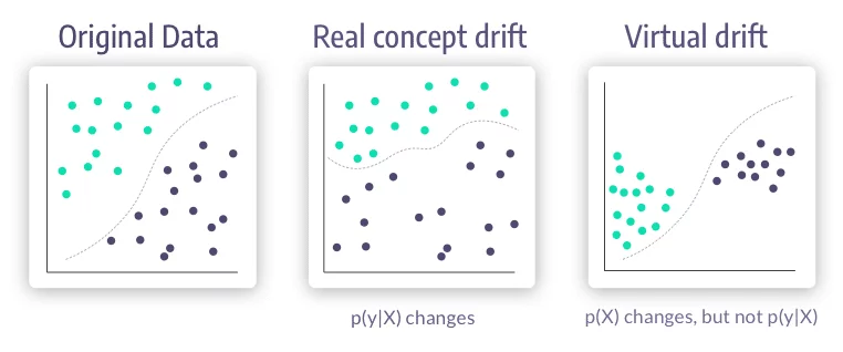
Concept Drift vs. Data Drift
Although “concept drift” refers specifically to the model's accuracy, most data science practitioners include virtual drift (sometimes called data drift) in that too.
To understand this in a statistical manner, given a sample instance X ∈ ci, we can try to classify it by:
![]()
Therefore, drift may occur in 3 ways:
- Class priors P(c) (how likely are we to see this class) changes while p(X|c) remains unchanged (this class has the same probability to produce this ).
- The input distribution p(X) changes (we receive different distribution of input feature vectors) while p(c|X) remains unchanged (population drift / covariate shift / data drift)
- Class definition change p(c|X) while p(X) remains the same. (real drift / concept drift / functional relation change)
Going back to the business level, we can see examples of drift in many use cases:
Wind power prediction: when predicting the electric power generated from wind from an off-line dataset based model, we have concept drift vs. on-line training models due to the non-stationary properties of winds and weather.
Spam detection: Email content and presentation change constantly (data drift). Since the collection of documents used for training changes constantly, the feature space representing the collection changes. Also, users themselves change their interests, causing them to start or stop considering some emails as spam (concept drift).
What does concept drift look like?
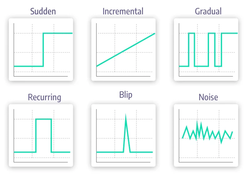
Concept drift changes can be:
Sudden: The move between an old concept to a new concept happens at once. The behavioral patterns associated with the COVID-19 pandemic have provided us with striking examples, like the lockdowns that abruptly changed population behaviours all over the world.
Incremental / Gradual: The change between concepts happens over time, as the new concept emerges and starts to adapt. The move from summer to winter could be an example of gradual drift.
Recurring / Seasonal: The changes re-occur after the first observed occurrence. The seasonal shift in weather, which dictates that consumers buy coats in colder months, cease these purchases when spring arrives and then begin again in the fall, is an example.
How we encounter drift in a specific use case can have a lot of influence over how it should be handled. If we expect sudden drifts in a particular use case, we may set a detection system for a rapid change in our features or predictions. However, if we use the same detectors in a gradual drift use case it will probably fail to detect the drift at all, and system performance will start to deteriorate.
What is a Drift Aware System?
If we simply deploy models to production without any monitoring system, we risk model performance deterioration over time due to concept drift. However, simply monitoring the data and acknowledging that some shift may have happened is only the first stage of building a drift-aware system.
There are four main parts of a drift-aware system:
- Change detection
- Memory
- Learning
- Loss estimation
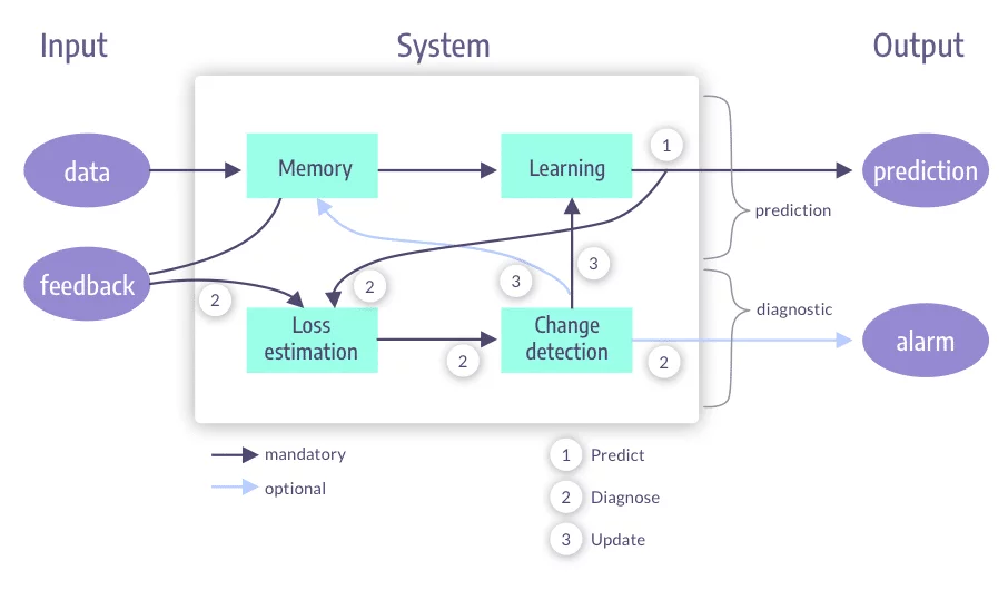
Change Detection
When our model is live in production, we can trigger an alarm for any type of relevant change, which in turn triggers a learning or memory process.
There are a few different methods that can be used to detect drift:
SPC / Sequential Analysis Concept Drift detectors
This family of detectors verifies that the model's error-rate is stable (in-control) and alerts when the error-rate is out-of-control. Some of the models even have a warning zone in between the modes that could enable us to flag the subsequent samples for later analysis and training.
Under this detector segment we can find methods such as:
DDM / EDDM (Early) Drift Detection Method: Models the number of errors as a binomial variable. This enables us to confine the expected number of errors in a prediction stream window to within some standard deviation. if ![]() and
and 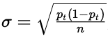 ), then we can alarm when:
 ![]() DDM, or use the distance between 2 consecutive errors
DDM, or use the distance between 2 consecutive errors ![]() 0.90 EDDM.
0.90 EDDM.
Note:
- EDDM is better than DDM for detecting gradual drift, but is more sensitive to noise.
- They both require a minimal number of errors to initialise their inner statistics.
LFR (Sequential Analysis): For stationary data, we would assume the contingency table (Confusion Matrix) to stay close to constant. Thus, we can calculate the 4 different rates:
![]() ,
, ![]() ,
, ![]() ,
, ![]() and perform Monte Carlo Sampling for significance levels and Bonferroni Correlation for correlated tests.
and perform Monte Carlo Sampling for significance levels and Bonferroni Correlation for correlated tests.
Page Hinkley test (PHT): A sequential analysis technique typically used for monitoring change detection in the average of a Gaussian signal. However, it is relatively robust in the face of non-normal distributions and has been recently applied to concept drift detection in data streams.
Monitoring Distributions Between Different Time Windows
In this family of detection methods, a sliding detection window is compared to a fixed reference window to test if the distributions match. Typically, the test dataset is taken as a reference point for the received input sliding window.
- Statistical Distribution Properties: Using distribution metrics such as KL- Divergence, Total Variation Distance, and Hellinger Distance. Note: These are great to use with input features.
- Adaptive Sliding Window (ADWIN): Given the window W, if the two sub windows W0,W1 are large enough and their means are different, we can drop W0 (the older) and note a change in distribution.
Contextual approaches
There are many different ways to test if the current data holds different signals than the training data, including the judicial use of some algorithms and their properties. For instance:
- Add the timestamp as a feature to a decision tree based classifier. If the tree spliced the data on the timestamp, it suggests a different context.
- Train a large stable model on the large dataset and a small reactive model on a new smaller window. If the recent reactive model outperforms the stable model, the latest window may hold new concepts.
Memory
When new data for prediction comes in, we need to consider how it will be used to train our model later on. Mechanisms such as online learning update the algorithm's knowledge for every sample it encounters, coupled with a forgetting mechanism to adapt to the latest concept changes.
We can train the model in batches (as is done in the majority of cases). In this situation, we need to plan for periodical updates to the model (re-training). How to select which new data to use in re-training? Use a fixed window (for example, of the last 3 months or latest 1M rows of data) and train on that every interval. Remember: smaller window sizes can learn new concepts faster but are also more susceptible to noise and lower performance in stable periods.
Variable window creates new datasets by examining the distributions rising from the data, thus creating a new dataset only when some change is detected (ADWIN).
To forget older data, sampling methods can be used, like taking the latest X period (thus abruptly forgetting anything that happened before), and creating an N samples dataset, sampled from different timeframes with some probability OR we can gradually forget by giving weight to samples according to a specified metric, for example: wλ(X) = exp(−λj) where we can give each passing day a linearly or exponentially smaller weight.
Learning
Once datasets for the models have been created, the next step is to combine learning components to generalize from the examples and update the predictive model from the evolving dataset. We will define:
- Learning mode: To update the model with new data.
- Model adaptation: To trigger a learning update by analyzing the model behavior over time-evolving data.
- Model management: To maintain active predictive models.
Learning Mode: Applying the New Data to the Learning Model
Retraining discards the current model and builds a new model from the buffered data. This can be done incrementally, or online (where the model is updated after each example). In online retraining, new data erases prior patterns over time.
Model Adaptation: When to Start the Learning Process and How to Manage the Change
There are a few different triggering mechanisms that can be used to start the learning process:
- Blind: Adapt the model without an explicit "concept drift" detection. For example, retrain every day, or every x samples. This usually uses some fixed window. Online algorithms are blind by default as they continuously learn with each sample. Therefore, they forget concepts at a fixed rate. For abrupt concept change, this may cause a lag in detection rather than retrain a model.
- Informed: These are reactive strategies that can be triggered by a drift detection system or a specific data descriptor.
Once an update has been triggered, the new model can be appended to the existing solution. Here too, there are a few options to accomplish this:
- Global replacement: Delete the old model and create a new one from scratch.
- Local replacement: Used mainly in online algorithms like a hoeffding tree, changes are made only to some splits, thus altering just the drift-affected region of the model.
- Ensemble models fit in here too: Part of the ensemble can be changed with the new model. It's important to take into account that as memory and computational resources are not infinite, new concepts cannot infinitely be added to the models and some replacement process is bound to happen at some point.
Model Management: Maintaining Active Models
Depending on the way the data behaves and how concepts appear and disappear from it, earlier models can sometimes be useful. So how do we manage all these models? Here are a few approaches:
- Ensembles enable us to deploy many adaptive strategies for dynamically changing data.
- When outdated models are discarded they can be put into "sleep mode". They can then be rechecked upon drift detection.
- Meta-learning schema can be used to identify possible candidate models.
Drift Aware Systems: Some Examples
There are many examples of drift-aware systems with different algorithmic traits and use cases.
Simple retraining: Using DDM / EDDM alerts, initiate a new model training process over the latest data window.
Smart(er) retraining: Using the change detection "warning zone", collect samples and append them to the training dataset. When a real alarm is received, train on the collected dataset.
Learn++: Train a new model on the latest data, add this model to the model’s ensemble and update the voting weight of each model.
Streaming Ensemble Algorithm (SEA): Train a new model on the latest batch of data (using any memory technique), add the new model to the model’s ensemble which is of fixed size and drop the lowest-performing model.
Dynamic Weighted Majority (DWM) / AddExp: For online models, maintain an ensemble of predictive models with weights (same algorithm but on different data), update the model voting weight by gamma for error / true prediction. If the overall prediction was wrong, add a new model, update the model weights and remove all models with weight under some threshold.
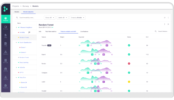
Deploy a Concept Drift Aware ML System with the Iguazio Data Science Platform
The Iguazio Data Science Platform contains all the necessary components to deploy an ML system to production easily and safely.
Using the V3IO Data Layer, Iguazio enables real-time collection of data including the incoming features, model predictions and relevant monitoring metrics produced in the process.
MLRun enables the easy deployment and orchestration of complex data and prediction pipelines. There are a few ensembles and integrated a few algorithms pre-built that you can take advantage of (check it out here), or extend with your own logic.
Iguazio’s integrated Grafana service contains monitoring dashboards pre-configured to track data and concept drift and you can customise your own alarms to only be alerted when needed.
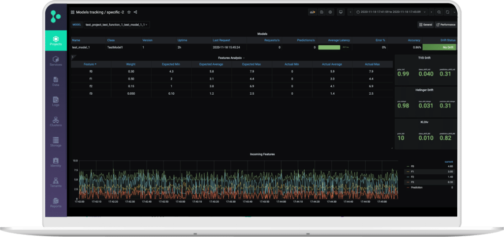
With all these components available out of the box and fully managed, ML teams can quickly build an end-to-end solution that covers the entire ML lifecycle, to drive faster innovation with better results over time.


