Integrating MLOps with MLRun and Databricks

How to train on Databricks and deploy with MLRun

Every organization aiming to bring AI to the center of their business and processes strives to shorten machine learning development cycles. Even data science teams with robust MLOps practices struggle with an ecosystem that is in a constant state of change and infrastructure that is itself evolving. Of course, no single MLOps stack works for every use case or team, and the scope of individual tools and platforms vary greatly.

Databricks is a hugely popular data platform with core ML capabilities, reportedly used by over 5000 enterprises. But for use cases requiring automation and scale, or complex use cases with real-time applications, data science teams may need some extra tooling for model serving. To understand why you might want that extra tooling, consider a complex but fairly common scenario: fetching historical data for the training side, with the security requirement that live data remains on-prem.

Databricks does offer real-time model serving capabilities, but by using MLRun real-time serving with the complex serving graph, you can deploy the real-time serving with pre-processing, model inference, post-processing in the same graph and scale different part of the graph independently.

In this blog post, I’ll show how to integrate models trained in Databricks and perform model serving with open-source tool MLRun.

Get Started with MLRun

Learn more about MLRun & how to quickly build and managing continuous ML and generative AI applications across their lifecycle.

Learn More

What is MLRun and the Iguazio MLOps Platform?

MLRun is a popular open-source MLOps framework that streamlines machine learning projects from data collection, experimentation, model development, feature creation, production model serving deployment and model monitoring, and full lifecycle management. The Iguazio MLOps Platform is built with MLRun at its core, with added enterprise features such as data management, user management, security, autoscaling, high availability, and more. With MLRun model serving, you can run your model inference, while abstracting away infrastructure management or scale constraints.

Check out MLRun documentation and the Iguazio MLOps Platform documentation to dive into all the details.

What is the Databricks Platform?

Databricks is a cloud-based platform for big data processing and analytics. It provides an integrated environment for running Apache Spark, their open-source data processing engine, as well as a suite of tools for working with data and developing machine learning models. Databricks also includes a collaboration and sharing platform for data scientists and engineers to work together and scale their work.

MLflow is an open source tool that comes built in to the Databricks platform, originally developed by Databricks for experiment tracking. While it now has additional functionality, this area is still where it really shines. It is a single Python package that covers some key steps in model management. For more details, check out their documentation here, learn more about the Databricks MLOps Stack (currently in private preview), and read our comparison blog covering MLflow, MLRun and Kubeflow.

Train and Track Models on Databricks

Databricks is a cloud-based platform for big data processing and machine learning. In Databricks, the data scientists can use Databricks notebooks as a development tool for data engineering, feature engineering, and model training.

Databricks provides a unified data platform that enables access to a wide variety of data sources such as databases, cloud storage, or Delta Lake, Databricks’ natively supported data in delta format.

In this post, we’ll take a theoretical use case of revenue prediction for a retail store, based on ad spending and several other factors (or features).  We will use a simple csv file as our data source. In a notebook, we will run through the steps of feature engineering so that the raw data will be transformed into features for the model training algorithm.

Data Engineering and Feature Engineering

Load data into pandas dataframe:

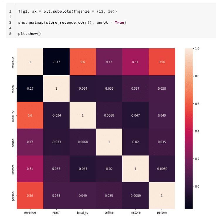
store_revenue = pd.read_csv('/dbfs/FileStore/datasets/store.csv')

Perform some exploration data analysis such as basic statics of the data set, using a heatmap to visualize the correlations of the features. For example, here is a heatmap plot from the dataset:

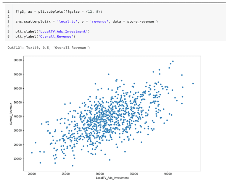
We can also visualize relationships using a scatter plot, for example, in the following scatter plot, a positive correlation is observed between investment in local ads and revenue:

In the raw data, there are some categorical variables which need to be converted into numerical values using a technics such as one-hot encode.

store_revenue = pd.get_dummies(store_revenue, columns = ['event'])

In addition to converting the categorical variable to the hot-encoded value, for the numerical variable, we also need to scale the variables made up of numerical columns from the training set and the test data.

scaler = StandardScaler()
X_train_numerical=pd.DataFrame(scaler.fit_transform(X_train_numerical), columns = X_train_numerical.columns)
X_test_numerical = pd.DataFrame(scaler.transform(X_test_numerical), columns = X_test_numerical.columns)

Combining our scaled numeric columns with our one-hot-encoded categorical columns (only the training dataset):

   X_train_categorical.reset_index(drop = True, inplace = True)
   X_train_numerical.reset_index(drop = True, inplace = True)
   X_train = pd.concat([X_train_numerical, X_train_categorical], axis = 1)

Combining our scaled numeric columns with our one-hot-encoded categorical columns (only the testing dataset)

     X_test_categorical.reset_index(drop = True, inplace = True)
     X_test_numerical.reset_index(drop = True, inplace = True)       
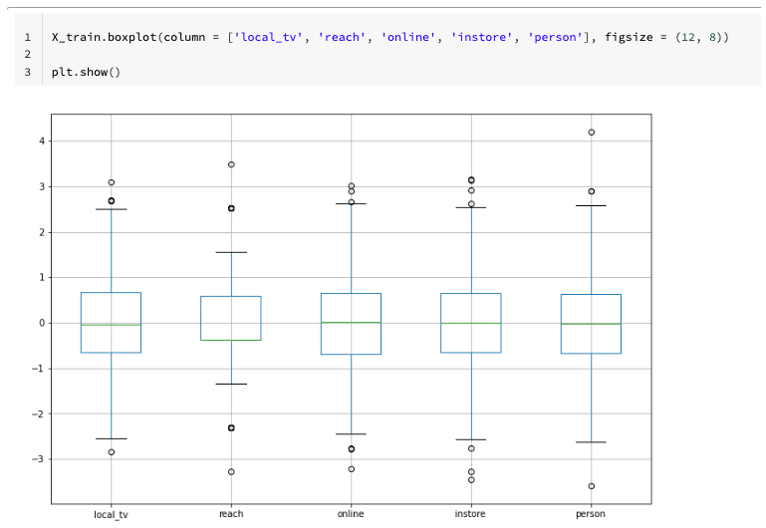
     X_test = pd.concat([X_test_numerical, X_test_categorical], axis = 1)

Post scaling, the numerical variables distributions can be seen in more or less the same range, see the boxplot below:

Experiment tracking

Databricks has MLflow built in, which covers experiment tracking, model management and more (to understand the differences between MLflow, MLRun and Kubeflow, check out our blog here). To track the model training, we will set the experiment first:

 mlflow.set_experiment(experiment_name) =        '/Users/xingshengq@iguazio.com/store_revenue_prediction')

To demonstrate the model ensemble later in the model serving part, we are going to train 3 different regression models.
The first model is going to be a linear regression model:

mlflow.sklearn.autolog() 
from sklearn.metrics import r2_score, mean_squared_error, mean_absolute_error 
with mlflow.start_run(run_name = 'linear_regression_model') as run1: 
      	    lr = LinearRegression() 
      lr.fit(X_train.values, y_train) 
      y_pred =  lr.predict(X_test) 
      testing_score = r2_score(y_test, y_pred) 
      mean_absolute_score = mean_absolute_error(y_test, y_pred) 
 
      mean_sq_error = mean_squared_error(y_test, y_pred) 
      run1 = mlflow.active_run() 
      print('Active run_id: {}'.format(run1.info.run_id))

The second model we are going to train is a random forest regressor:

with mlflow.start_run(run_name = 'randomforest_regression_model') as run2:

rf = RandomForestRegressor()

rf.fit(X_train.values, y_train)

y_pred =  rf.predict(X_test)

testing_score = r2_score(y_test, y_pred)

mean_absolute_score = mean_absolute_error(y_test, y_pred)

mean_sq_error = mean_squared_error(y_test, y_pred)

run2 = mlflow.active_run()

print('Active run_id: {}'.format(run2.info.run_id))

Train the third model, a k-nearest neighbors regression model:

with mlflow.start_run(run_name = 'knn_regression_model') as run3:

      knn = KNeighborsRegressor()

      knn.fit(X_train.values, y_train)

      y_pred =  knn.predict(X_test)

      testing_score = r2_score(y_test, y_pred)

      mean_absolute_score = mean_absolute_error(y_test, y_pred)

      mean_sq_error = mean_squared_error(y_test, y_pred)

      run3 = mlflow.active_run()

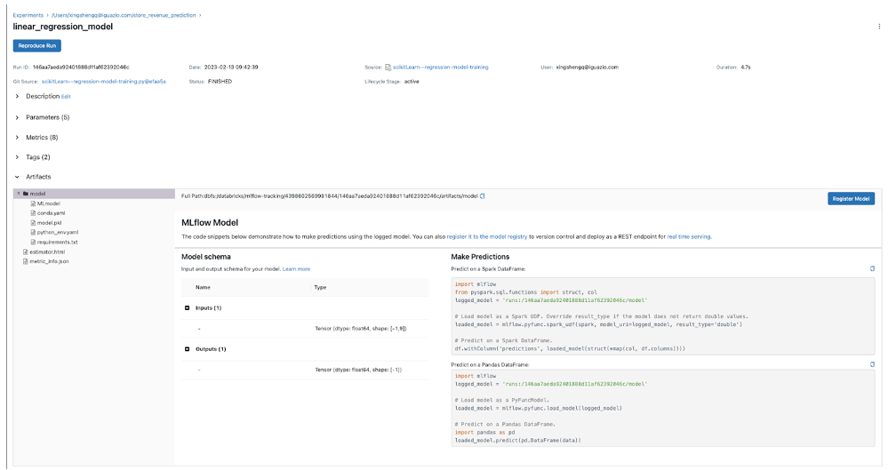
      print('Active run_id: {}'.format(run3.info.run_id))

After running the model training on the Databricks cluster, you can view the tracked experiment runs and the logged artifacts such as the models.

Copy the Trained Models to MLRun

MLRun is an open MLOps orchestration framework for quickly building and managing continuous ML applications across their lifecycle. MLRun integrates into your development and CI/CD environment and automates the delivery of production data, ML pipelines, and online applications. It provides a simple and efficient way to run and manage your ML workflows and pipelines, using Jupyter notebooks as the main development environment.

Using MLRun with Jupyter notebooks allows you to have the best of both worlds: you can use the power of Jupyter notebooks for interactive development and experimentation, and the efficiency and scalability of MLRun for deploying your models in production.

From an MLRun Jupyter notebook, you can download the models trained on a Databricks cluster using MlflowClient. To access to the Databricks from a MLRun Jupyter notebook, you’ll need to first configure the authentication to the cluster either with:

import os

os.environ['MLFLOW_TRACKING_URI'] = "databricks"

os.environ['DATABRICKS_HOST'] = "<your-databricks-host>"

os.environ['DATABRICKS_TOKEN'] = "<your-databricks-token>"

or you can set the env variables via:

export MLFLOW_TRACKING_URI=databricks

export DATABRICKS_HOST=<your-databricks-host>>

export DATABRICKS_TOKEN=<your-databricks-token>

With the authentication set up, you can copy the trained models for a specific the run-id. Here is a snippet showing how to copy the models for a run-id to a destination on the MLRun cluster. In this example, we will save the model to a local directory for simplicity.

# Download artifacts

client = MlflowClient("databricks")

local_dir = "./linear_regression_model"

if not os.path.exists(local_dir):

    os.mkdir(local_dir)

local_path = mlflow.artifacts.download_artifacts(run_id="859e433b50ae46a9a8818d1877ec1fcc", dst_path=local_dir)

print("Artifacts downloaded in: {}".format(local_path))

print("Artifacts: {}".format(os.listdir(local_path)))

Deploy Model Inference on MLRun

To deploy a machine learning model for inference using MLRun, you need to follow these steps:

1. Create a function that loads your model and performs inference. This function should take input data as an argument, run inference using the model, and return the output.
2. Use the MLRun API to create an MLRun function that implements the inference function you created in step above. MLRun functions are reusable, versioned, and can be invoked from any environment, including Jupyter notebooks, web applications, or other MLRun functions.
3. Use the MLRun API to deploy the function. MLRun will automatically create a container image with your function and deploy it to a Kubernetes cluster.
4. Use the MLRun API you can test the deployed function, by sending sample input data to the function and checking the output.
5. Once you have verified that your function is working correctly, you can use it in your applications or other MLRun functions, by invoking it using the MLRun API.

By using MLRun to deploy your machine learning models, you can easily manage, version, reuse your models, and scale your inference workloads as needed. Additionally, MLRun provides advanced features, such as automatic scaling, monitoring, and tracing, that make it easier to run and manage your ML workflows and pipelines at scale.

When you deploy a model inference, you can include steps for data pre-processing, model results post-processing, model chaining, or model ensemble in the inference pipeline. Next, I will walk through the steps in a notebook to deploy a model inference function to an MLRun cluster with a model ensemble that will generate model predictions and combine the model predictions according to your ensemble mechanism.

Define Functions and Classes Used in the Model Serving Graph:

from cloudpickle import load

from typing import List

from sklearn.datasets import load_iris

import numpy as np

import mlrun

# model serving class example

class RegressionModel(mlrun.serving.V2ModelServer):

    def load(self):

        """load and initialize the model and/or other elements"""

        model_file, extra_data = self.get_model('.pkl')

        self.model = load(open(model_file, 'rb'))

    def predict(self, body: dict) -> List:

        """Generate model predictions from sample."""

        feats = np.asarray(body['inputs'])

        result: np.ndarray = self.model.predict(feats)

        return result.tolist()

# echo class, custom class example

class Echo:

    def __init__(self, context, name=None, **kw):

        self.context = context

        self.name = name

        self.kw = kw

    def do(self, x):

        print("Echo:", self.name, x)

        return x

# error echo function, demo catching error and using custom function

def error_catcher(x):

        x.body = {"body": x.body, "origin_state": x.origin_state, "error": x.error}

        print("EchoError:", x)

        return None

Create a New Serving Function Within a Serving Graph:

function = mlrun.code_to_function("advanced", kind="serving",

                                  image="mlrun/mlrun",

                                  requirements=['storey'])

graph = function.set_topology("flow", engine="async")

path1 = '/User/blog/databricks-mlrun/linear_regression_model/model/model.pkl'

path2 = '/User/blog/databricks-mlrun/knn_regression_model/model//model.pkl'

path3 = '/User/blog/databricks-mlrun/randomforest_regression_model/model/model.pkl'

# use built-in storey class or our custom Echo class to create and link Task states

graph.to("storey.Extend", name="enrich", _fn='({"tag": "something"})') \

     .to(class_name="Echo", name="pre-process", some_arg='abc').error_handler("catcher")

# add an Ensemble router with two child models (routes). The "*" prefix mark it is a router class

router = graph.add_step("*mlrun.serving.VotingEnsemble", name="ensemble", after="pre-process")

router.add_route("m1", class_name="RegressionModel", model_path=path1)

router.add_route("m2", class_name="RegressionModel", model_path=path2)

router.add_route("m3", class_name="RegressionModel", model_path=path3)

# add the final step (after the router) that handles post processing and responds to the client

graph.add_step(class_name="Echo", name="final", after="ensemble").respond()

# add error handling state, run only when/if the "pre-process" state fails (keep after="") 

graph.add_step(handler="error_catcher", name="catcher", full_event=True, after="")

# plot the graph (using Graphviz) and run a test

graph.plot(rankdir='LR')

You can view the model serving graph here:

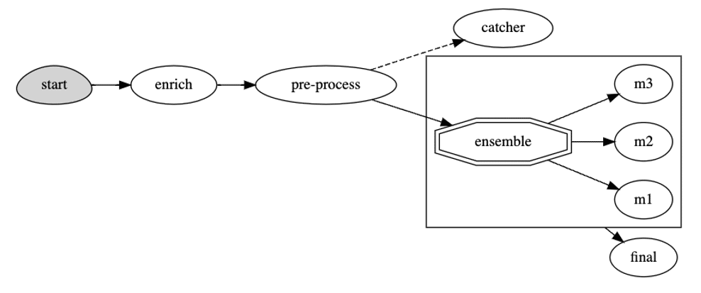
As you can see, the serving graph includes some pre-processing and model ensemble in the pipeline. Note that you can implement your own ensemble logic if you need, in this example, the default ensemble logic is the mean of the output from all the models for the regression model.

Test a Serving Graph Locally on a Jupyter Notebook

Load in some sample data for testing:

x=[[1.552441,0.385221,1.756843, -0.136519, 0.631093,0.0,0.0,1.0,0.0],

    [1.552441,0.500727,-0.372055,0.487178,-0.993654,0.0,0.0,0.0,1.0],

    [1.552441,-0.997883,-0.148913,-0.970829,1.280992,0.0,0.0,0.0,1.0],

    [0.588006,1.107827,-0.896741,-0.685943,0.306143,0.0,0.0,0.0,1.0],

    [-0.376428,-1.270696,0.675306,-0.711379,-0.668705,1.0,0.0,0.0,0.0]  

  ]

print(x)

server = function.to_mock_server()

resp = server.test("/v2/models/infer", body={"inputs": x})

server.wait_for_completion()

resp

Here are the test results:

{'id': '30a20d4f830044cfafa4358c465dbc80',

 'model_name': 'ensemble',

 'outputs': [43156.66223187226,

  36374.07433613021,

  34362.53904014997,

  42372.60100852936,

  25498.259322385],

 'model_version': 'v1'}

Deploy the Serving Graph as a Real-Time Serverless Function:

Run the function deploy to deploy the serving graph onto the MLRun cluster and will give us an endpoint URL for model inference.

from mlrun.platforms import auto_mount

function.apply(auto_mount())

url=function.deploy()

> 2023-02-13 19:42:25,495 [info] successfully deployed function: {'internal_invocation_urls': ['nuclio-default-advanced.default-tenant.svc.cluster.local:8080'], 'external_invocation_urls': ['default-advanced-default.default-tenant.app.us-sales-350.iguazio-cd1.com/']}

'http://default-advanced-default.default-tenant.app.us-sales-350.iguazio-cd1.com/'

We can either use MLRun function invoke API to call the inference:

function.invoke("/v2/models/infer", body={"inputs": x})

{'id': '8344050d-f44e-4932-9080-ce17a1ec2fed',

 'model_name': 'ensemble',

 'outputs': [43156.66223187226,

  36374.07433613021,

  34362.53904014997,

  42372.60100852936,

  25498.259322385],

 'model_version': 'v1'}

or through HTTP endpoint like this:

import requests

resp = requests.put(url + '/v2/models/infer', json={"inputs": x})

print(f'Model Name: {resp.json()["model_name"]}')

print(f'Model Version: {resp.json()["model_version"]}')

print(f'Model Outputs: {resp.json()["outputs"]}')

Model Name: ensemble

Model Version: v1

Model Outputs: [43156.66223187226, 36374.07433613021, 34362.53904014997, 42372.60100852936, 25498.259322385]

Summary

In this post, we walked through the steps to:

• Train and track machine learning models in the Databricks cluster
• Copy the models from Databricks to an MLRun cluster
• Create a serving graph in the MLRun cluster and deploy the serving function for the model inference
• Run the simple inference testing with the serving function as well using the model serving HTTP endpoint.

The goal of this post is to show how a machine learning project can take advantage of different toolsets and purpose-built platforms to streamline the MLOps process. There may be use cases where you can use the historical data for the model training in Databricks but we can’t move the realtime data into the cloud for inference due to data security requirements. MLRun can run the model serving in cloud or on-prem, provides a great solution for the restrictions. This example shows how to use Databricks for model training and tracking while using MLRun to deploy model serving. In addition to the easy deployment of model serving in an MLRun cluster, there are many more features within the MLRun framework, such as automated offline and online feature engineering for real-time and batch data, the rapid development of scalable data and ML pipelines using real-time serverless technology, codeless data and model monitoring, drift detection and automated re-training, and integrated CI/CD across code, data, and models, using mainstream Git and CI/CD frameworks.

Questions? Feel free to reach out to us on the MLOps Live Slack community in the #mlrun channel.