The Complete Guide to Using the Iguazio Feature Store with Azure ML - Part 4
Nick Schenone | February 2, 2022
Hybrid Cloud + On-Premises Model Serving + Model Monitoring
Recap
Last time in this blog series, we provided an overview of how to leverage the Iguazio Feature Store with Azure ML in part 1. We built out a training workflow that leveraged Iguazio and Azure, trained several models via Azure's AutoML using the data from Iguazio's feature store in part 2. Finally, we downloaded the best models back to Iguazio and logged them using the experiment tracking hooks in part 3.
In this final blog, we will:
- Discuss the benefits of a hybrid cloud architecture
- Define model load and predict behavior
- Create a model ensemble using our top three trained models
- Enable real-time enrichment via the feature store during inferencing
- Deploy our model ensemble in a Jupyter notebook and on a Kubernetes cluster
- Enable model monitoring and drift detection
- View model/feature drift in specialized dashboards
Hybrid Cloud Benefits and Motivation
Hybrid clouds are all the rage. While cloud computing has given many organizations access to near infinite compute power, the reality is that on-premise infrastructure is not going away. From data privacy concerns, to latency requirements, to simply owning hardware, there are many legitimate reasons for having an on-premise footprint.
However, with this increased flexibility comes increased complexity – the right tools are needed for the job. With the multitude of end-to-end platforms, SaaS services, and cloud offerings, it is increasingly difficult to find those correct tools—especially those that work across cloud and on-premise environments.
In the last blog of this series, we will combine the feature store and on-premise model serving of the Iguazio MLOps Platform with the models trained via Azure’s AutoML to create a full end-to-end hybrid cloud ML workflow.
Define Model Behavior
Now that we understand the motivation behind the on-premise deployment, the first step to deploying our models is to define the inferencing behavior. Essentially, how do we load our model and use it for predictions? MLRun Serving Graphs allow users to define a high level Python class for these behaviors, much like KFServing and Seldon Core.
Since all the models we downloaded from AzureML are pickle files and have the same prediction syntax, this is a very straightforward class. The inferencing class resides in the azure_serving.py file and includes the following:
import numpy as np
from cloudpickle import load
from mlrun.serving.v2_serving import V2ModelServer

class ClassifierModel(V2ModelServer):

    def load(self):
        """load and initialize the model and/or other elements"""
        model_file, extra_data = self.get_model('.pkl')
        self.model = load(open(model_file, 'rb'))

    def predict(self, body: dict) -> list:
        """Generate model predictions from sample"""
        print(f"Input -> {body['inputs']}")
        feats = np.asarray(body['inputs'])
        result: np.ndarray = self.model.predict(feats)
        return result.tolist()
Note that your class can be as complex as you need it to be with built-in hooks for preprocessing, post processing, validation, and more. For more information on MLRun Serving Graphs, check out the documentation.
Define Serving Function
After writing our simple Python class, the MLRun framework will take care of the building, provisioning, routing, enriching, aggregating, etc.
First we will configure our code to use the same project that our features and models reside in:
import os
from mlrun import get_or_create_project, code_to_function

project = get_or_create_project(name="azure-fs-demo", context="./")


Like in the previous blog, we will be using MLRun's code_to_function capabilities to containerize and deploy our function. However, unlike last time, we will be using a different runtime engine. Instead of a batch job, we will be deploying a model serving function:
serving_fn = code_to_function(
    name='model-serving',                # Name for function in project
    filename="azure_serving.py",         # Python file where code resides
    kind='serving',                      # MLRun Serving Graph
    image="mlrun/mlrun",                 # Base Docker image
    requirements="requirements.txt"      # Required packages
)
Configure Model Ensemble with Feature Store Enrichment
In addition to the initial code_to_function configuration, we will be adding additional options to the serving function. Behind the scenes, we are really constructing a graph with different topologies, preprocessing steps, models, etc.
In our case, we are looking for a model router that can do the following:
- Enrich incoming data using the feature store
- Impute any missing values using statistics from the feature store
- Utilize multiple models in a voting ensemble
- Return a single result from the ensemble
MLRun has such a router that comes out of the box called the EnrichmentVotingEnsemble. The configuration looks like the following:
serving_fn.set_topology(
    topology='router',
    class_name='mlrun.serving.routers.EnrichmentVotingEnsemble',
    name='VotingEnsemble',
    feature_vector_uri="heart_disease_vec",
    impute_policy={"*": "$mean"}
)
Notice that we are configuring the desired FeatureVector to enrich with as well as the imputation method for missing values.
Now that the model router is set up like we want, we can add our models. We will be referencing the models using their URI’s available via the MLRun UI. The “copy URI” icon is circled in red below:
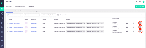
We can add the models using very simple syntax. This sets the name of the model in the graph, the desired Python class to use for load/predict behavior, as well as the path to the model itself (using the URI we copied). This looks like the following:
serving_fn.add_model(

    key="model_0",
    class_name="ClassifierModel",
    model_path="store://models/azure-fs-demo/model_0_svcwrapper#0:latest"
)
serving_fn.add_model(
    key="model_1",
    class_name="ClassifierModel",
    model_path="store://models/azure-fs-demo/model_1_logisticregression#0:latest"
)
serving_fn.add_model(
    key="model_2",
    class_name="ClassifierModel",
    model_path="store://models/azure-fs-demo/model_2_logisticregression#0:latest"
)
Finally, we can save our serving function in our project and visualize the computation graph:
serving_fn.save()
serving_fn.spec.graph.plot()
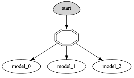
Before continuing, consider the complexity of what we just set up using a few lines of code:
- Define model load and predict behavior
- Create a model ensemble using our top 3 trained models
- Enable real-time enrichment via the feature store during inferencing
- Enable real-time imputation of missing values using feature store statistics
Test Locally in Jupyter Notebook
Now that our serving function and model ensemble are setup, we should test it out in our local Jupyter environment. MLRun makes this quite simple to do:
from azure_serving import ClassifierModel      # Need our serving class available for local server

local_server = serving_fn.to_mock_server()     # Create local server for testing


> 2021-12-15 23:08:35,858 [info] model model_0 was loaded
> 2021-12-15 23:08:35,931 [info] model model_1 was loaded
> 2021-12-15 23:08:36,000 [info] model model_2 was loaded
From here, we can invoke the model using one of the patient_ids from our dataset. This will:
- Retrieve the corresponding record in the feature store
- Impute any missing values
- Send the fully enriched record to our model ensemble
- Aggregate and return the results of the model ensemble
This looks like the following:
local_server.test(
    path='/v2/models/infer',
    body={
        'inputs': [
            ["d107db82-fe26-4c02-b264-a3749510ed9b"]
        ]
    }
)


Input -> [[0, 0, 1, 0, 62, 0, 1, 1, 0, 0, 0, 138, 294, 0, 1, 1, 106, 1, 0, 1.9, 0, 0, 1, 3.0, 0, 1, 0]]
Input -> [[0, 0, 1, 0, 62, 0, 1, 1, 0, 0, 0, 138, 294, 0, 1, 1, 106, 1, 0, 1.9, 0, 0, 1, 3.0, 0, 1, 0]]
Input -> [[0, 0, 1, 0, 62, 0, 1, 1, 0, 0, 0, 138, 294, 0, 1, 1, 106, 1, 0, 1.9, 0, 0, 1, 3.0, 0, 1, 0]]
{'id': 'e36dedd8c72c48c48ff01594064c84fa',
 'model_name': 'VotingEnsemble',
 'outputs': [0],
 'model_version': 'v1'}
Not only do we receive the desired prediction and model information, we also see that the fully enriched record is printed out three times. This is due to the print statement in our predict function in azure_serving.py being called for each of our three models.
Now that we have verified that our model ensemble is working as expected in our Jupyter environment, we need to deploy it on our Kubernetes cluster.
Enable Model Monitoring
In addition to the deployment itself, we want to enable model monitoring and drift detection on our serving function. There are many excellent resources available on why model monitoring is important as well as how to build a drift-aware ML system. This is not a trivial task, especially for online drift calculations using real-time production data.
Luckily for us, this is available out of the box using the Iguazio platform. Behind the scenes, Iguazio will be deploying a real-time stream processor as well as an hourly scheduled batch job to calculate drift. The architecture looks something like this:
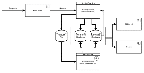
However, for our purposes, we don't need to worry about any of that. We can simply enable model monitoring for our serving function with the following snippet:
serving_fn.set_tracking()
project.set_model_monitoring_credentials(os.getenv('V3IO_ACCESS_KEY'))
Deploy on Kubernetes Cluster
Finally comes the moment of truth - production deployment on Kubernetes. In many cases, this is where projects go to die. In fact, some estimate that 85% of AI projects fail moving between development and production.
Not for us. Because we are using MLRun for containerization/configuration/deployment, we are almost done with our journey. To do the final deployment, we run this single line:
serving_fn.deploy()


> 2021-12-15 20:33:41,122 [info] Starting remote function deploy
2021-12-15 20:33:42  (info) Deploying function
2021-12-15 20:33:42  (info) Building
2021-12-15 20:33:43  (info) Staging files and preparing base images
2021-12-15 20:33:43  (info) Building processor image
2021-12-15 20:33:44  (info) Build complete
2021-12-15 20:33:51  (info) Function deploy complete
> 2021-12-15 20:33:52,276 [info] successfully deployed function: {'internal_invocation_urls': ['nuclio-azure-fs-demo-model-serving.default-tenant.svc.cluster.local:8080'], 'external_invocation_urls': ['azure-fs-demo-model-serving-azure-fs-demo.default-tenant.app.XXXXXXX.XXXXXXX.com/']}
This will build a new Docker image using the base image/requirements we specified, followed by deploying our serving graph to a real-time Nuclio function. Additionally, it will automatically deploy the stream/batch processor for model monitoring purposes.
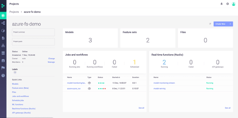
We can see these changes displayed in the MLRun project UI:
We can test our newly deployed function using the default HTTP trigger like so:
serving_fn.invoke(
    path='/v2/models/infer',
    body={
        'inputs': [
            ["d107db82-fe26-4c02-b264-a3749510ed9b"],
            ["4d05f307-b699-4dbe-b51d-f14627233e5a"],
            ["43f23da3-99d0-4630-9831-91d7b54e757e"],
            ["e031ed66-52f8-4f49-9881-aeff00be2be1"],
            ["31ff724d-b29b-4edb-9f70-f4da66902fe2"]
        ]
    }
)


> 2021-12-15 20:33:56,189 [info] invoking function: {'method': 'POST', 'path': '<http://nuclio-azure-fs-demo-model-serving.default-tenant.svc.cluster.local:8080/v2/models/infer>'}
{'id': 'f178c7da-0dd7-4d1b-8049-5328231229d7',
 'model_name': 'VotingEnsemble',
 'outputs': [0, 1, 1, 0, 1],
 'model_version': 'v1'}
The default invocation trigger is via HTTP, but we can also add additional triggers like Cron, Kafka, Kinesis, Azure Event Hub, and more
Simulate Production Traffic
Before viewing our model monitoring dashboards, we need something to monitor. We are going to simulate production traffic by continuously invoking our function using the patient_ids from our FeatureVector.
We can retrieve a list of the patient_ids like so:
import mlrun.feature_store as fstore

records = fstore.get_offline_features(
    feature_vector="azure-fs-demo/heart_disease_vec",
    with_indexes=True
).to_dataframe().index.to_list()
Then, we can invoke our serving function with random records and delays like so:
from random import choice, uniform
from time import sleep

for _ in range(4000):
    data_point = choice(records)
    try:
        resp = serving_fn.invoke(path='/v2/models/predict', body={'inputs': [[data_point]]})
        print(resp)
        sleep(uniform(0.2, 1.7))
    except OSError:
        pass


> 2021-12-15 21:37:40,469 [info] invoking function: {'method': 'POST', 'path': '<http://nuclio-azure-fs-demo-model-serving.default-tenant.svc.cluster.local:8080/v2/models/predict>'}
{'id': '65e2c781-31e5-46de-8e1d-2254d7c1b8af', 'model_name': 'VotingEnsemble', 'outputs': [1], 'model_version': 'v1'}
> 2021-12-15 21:37:41,707 [info] invoking function: {'method': 'POST', 'path': '<http://nuclio-azure-fs-demo-model-serving.default-tenant.svc.cluster.local:8080/v2/models/predict>'}
{'id': 'da267484-3b00-4752-87a9-157e2e3ca31c', 'model_name': 'VotingEnsemble', 'outputs': [1], 'model_version': 'v1'}
> 2021-12-15 21:37:43,411 [info] invoking function: {'method': 'POST', 'path': '<http://nuclio-azure-fs-demo-model-serving.default-tenant.svc.cluster.local:8080/v2/models/predict>'}
{'id': '4502196f-b9bb-45ea-a909-22670aa4cc58', 'model_name': 'VotingEnsemble', 'outputs': [0], 'model_version': 'v1'}
View Monitoring Dashboards
Once our simulated traffic has run for a bit, we can check our model monitoring dashboards.
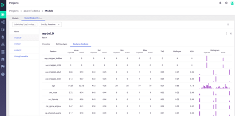
The first dashboard is high level drift information in the MLRun Project UI.
Here we can see statistics, histogram, and drift metrics per feature.:
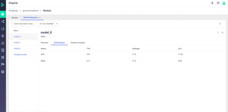
We can also view overall model drift analysis:
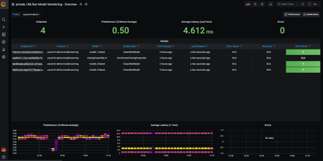
The second dashboard is more in depth drift and inferencing information in a Grafana dashboard.
Here we can see drift per model, average number of predictions, and average latency per project:
We can also view a graph of incoming features over time. This is one of my personal favorite dashboards as it lets you visualize how your incoming features change over time:
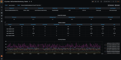
Finally, you can see model performance, latency, drift metrics over time, and any custom metrics you are logging:
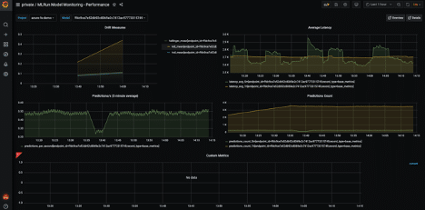
All of these dashboards and visualizations come out of the box with little to no additional configuration required.
If and when model drift is detected, an event with the drift information will be posted to a stream. From there, we can add consumers to the stream to perform tasks like sending notifications or kicking off a re-training pipeline.
Closing Thoughts
In this blog series, we have accomplished a lot. Using a combination of the Iguazio MLOps platform and Azure's AutoML capabilities, we have created a full end-to-end training flow that does the following:
- Ingest and transform dataset into feature store
- Upload/register features from Iguazio feature store into Azure ML
- Orchestrate Azure AutoML training job from Iguazio platform
- Download trained model(s) + metadata from Azure back into Iguazio platform
- Deploy top 3 models in model ensemble to real-time HTTP endpoint
- Integrate model serving with real-time enrichment and imputation via feature store
- Integrate model serving with model-monitoring and drift-detection
This whole flow is reproducible and modular in nature—meaning it would be simple to add additional steps, datasets, models, etc.
If you are interested in learning more about the integration between Iguazio and Azure AutoML, please check out our documentation, request a free trial, or reach out to our team of experts today!

