Classification is the set of algorithms that, together with regression, comprises supervised machine learning (ML). Supervised ML provides predictions on data. These predictions can take the form of a discrete class or a continuous value. Discrete use cases are the remit of classification (e.g., yes/no or true/false predictions), and continuous use cases fall under regression (such as propensity scores or price predictions).
This article presents an introduction to the classification threshold in ML, a discussion of the importance of tuning it to each use case, and a case study of how to choose the best threshold value.
Classification tasks are binary when there are two classes to predict on, or multi-class when there are more than two classes. Most classification algorithms can be used for either, with one main difference: The activation function. Most commonly, the sigmoid function is used for binary classification, and the softmax function for multi-class classification.
The sigmoid function outputs the probability between 0 and 1 for the positive class, i.e., the most relevant class for which we are predicting. The softmax function is a generalization of the sigmoid to additional classes, and it outputs a probability for each class. While the two functions return the same value for the positive class in binary classification, the sigmoid is most often used in practice because it is less expensive to calculate and operates more seamlessly than the softmax.
To derive the actual predicted class from the real output of the sigmoid, we apply a threshold that differentiates between the two. By default, this classification threshold is set to 0.5. This means that any prediction above 0.5 belongs to the positive class and anything below 0.5 to the negative class. How we set the classification threshold can make a real difference in the model’s performance.
The classification threshold in ML, also called the decision threshold, allows us to map the sigmoid output of a binary classification to a binary category.
Let’s take an example of logistic regression applied to spam detection, where the two classes are spam and non-spam. Logistic regression with the sigmoid returns a probability between 0 and 1 for an input data sample to belong to the positive class. A probability of 0.99 means that the email is very likely to be spam, and a probability of 0.003 that it is very likely to be non-spam. If the probability is 0.51, the classifier is less able immediately to determine the nature of the email.
We have to define a reliable threshold for the classifier that clearly indicates the split between the two classes. The ML threshold for most algorithms is set to 0.5 by default. Under this default, we’d classify the previous example as spam.
It can be risky to assume that the default 0.5 classification threshold is correct for a specific use case without proper model evaluation and analysis. The number and nature of model misclassifications will determine a machine learning initiative’s success. Setting the appropriate classification threshold is essential to limiting these misclassifications, and therefore indispensable in ML.
Some signs to look out for that indicate that 0.5 may not be the best threshold value include:
Various techniques exist to compensate for these cases by looking at improving the underlying data via preprocessing and augmentation, or by improving the algorithm itself with, for example, a custom loss function.
Classification thresholding is often preferred in practice as more interpretable and seamless. It is this option that we will focus on for the rest of the article.
The predicted labels for a binary classification task can map onto real labels in four different ways, as summarized by the confusion matrix (Figure 1).
Figure 1: The confusion matrix shows the mapping between predicted and true labels.
Correct predictions can be true positives (TP) or true negatives (TN), and misclassifications can be false positives (FP) or false negatives (FP). The positives are associated with the positive class, i.e., the class that we are interested in, and the negatives with the negative class, which can be seen as representing standard, less relevant behavior.
The classification threshold selection directly affects these values of the confusion matrix.
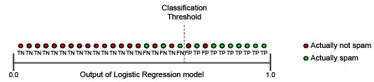
Figure 2: Visual representation of the relationship between classification threshold and prediction outputs (source: Google)
Depending on the objectives of the specific ML application, we will select a threshold that penalizes false negatives or false positives in this compromise. For our spam detection example, we prefer to minimize false positives in order to make sure that all relevant emails are in the user’s inbox, even if it means letting some spam find its way into their inbox too.
All ML classification thresholds are specific to their use case and must be tuned for each ML application individually. To choose the best classification threshold, we need to define what types of mistakes are least problematic to our use case (such as permitting false positives in our spam filter example).
While no ML model is perfect, we can make smart choices to optimize performance. One such optimization choice is tuning the classification threshold.
The most common method for classification threshold selection is plotting the ROC curve. ROC, which stands for receiver operating characteristic, plots the true positive rate (TPR=TPTP + FN) and false positive rate (FPR=FPFP + TN) at all classification thresholds.
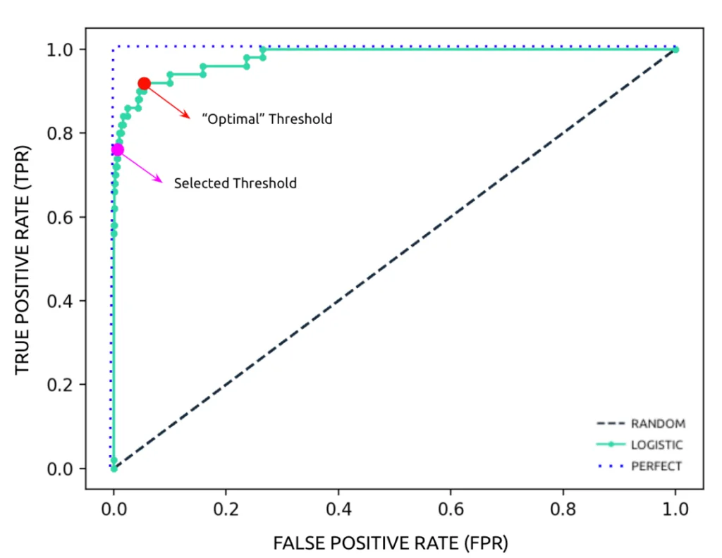
Figure 3: ROC curve for random and logistic regression classifiers
The ROC curve gives a quick visual understanding of the classifier’s accuracy. The closer to a right angle the curve, the more accurate the model. The classification threshold that returns the upper-left corner of the curve—minimizing the difference between TPR and FPR—is the optimal threshold.
As previously highlighted, false positives and false negatives most often don’t have the same relevance for a particular use case. We want to select a threshold that provides TPR at the maximum acceptable FPR, or vice versa. The selected threshold is frequently not the optimal threshold, and requires us to supplement it with other selection approaches.
Additional methods to select the desired threshold value in include:
While performing experimentation for classification threshold selection, we recommend keeping track of all runs and artifacts for reproducibility, collaboration, and efficiency.
MLRun is a useful tool for experiment tracking with any framework, library, or use case, and can be deployed as part of Iguazio’s MLOps platform for end-to-end data science.